Tom Judd <<<>>> Algorithms
Algorithms for Magnetic Compass Calibrations
Calibration Theory
The earth's magnetic field should be locally constant. Whatever the orientation of a platform with magnetic sensors, the reported magnitude of the magnetic field should be the same. In two dimensions, an unperturbed compass will report a constant field in all directions. Plotting the data will produce a circle centered at the origin. But when those sensors are stuffed into a device that has nearby ferromagnetic materials, the local magnetic field may be perturbed so that we do not see that symmetry in the response. Local material may be magnetized. This can add a constant vector to the earth's field. It will enhance the field when the earth's field is aligned with the local field, but will subtract from that field when it is aligned against the local field. That set of data will still be circular, but shifted away from the center by the magnitude of the perturbing field. This is a Hard Iron error.
Even un-magnetized materials have an effect. They serve as conduits for magnetic lines of flux. The resulting field can be enhanced or shielded along one direction. In two dimensions, the plotted data will be elliptical. This is a Soft Iron error. The major axes will not necessarily be aligned with our coordinate system.
It is quite common to have significant errors from both hard and soft perturbations. In two dimensions that would be an off-center tilted ellipse. In 3D it is an ellipsoid. The sample diagram of a 3D ellipsoid is taken from the 1985 patent of Marchent and Foster [4]. They developed the classic process of calibrating a 3D compass as follows:
Classic 3D Compass Calibration Process
- Solve for the polynomial coefficients of a 3D ellipsoid e.g.
A x2 + B y2 + C z2 + D x y + E x z + F y z + G x + H y + I z = 1
Each observed data point provides one set of x, y, and z for the equation. With nine unknowns, we need at least nine well placed data points to solve for the coefficients. - Solve for the center of the ellipsoid from the solution.
- Subtract the center from the solution (offsets px,py,pz in the diagram). This moves the ellipsoid to the origin of our coordinate system
- Solve for the eigenvalues and eigenvectors of the centered ellipsoid. The eigenvalues are the axis gains. The eigenvectors form a rotation matrix which defines the orientation of the ellipsoid
- Form the transformation matrix T from the gains G and orientation matrix R:
T = RT (A G-1/2 ) R
where A is a normalization constant and G-1/2 is a diagonal matrix whose elements are the recipricol sqrare roots of the gains. The transformation matrix plus the offsets when applied to the observed data, will correct for the perturbations that generated the ellipsoid. Note that you have to subtract the offsets first before applying any rotation.
There is no constraint that forces the above equation converge on an ellipsoid. With sparse or noisy data we could find ourselves with a 3D hyperbola. Refinements can force the solution to be an ellipsoid.[5][6]. These methods can pull a solution out of data where other algorithms fail. Nevertheless, bad, incomplete, or noisy data will always degrade the results. These techniques are moot when the goal is a precision compass.
No Calibration Table
Notice that there is no mention of a reference platform or calibration table in the above process. That is because you do not need a reference platform to calibrate a magnetic compass. A calibration table is needed in the factory to develop algorithms and to validate their effectiveness. But in the field, users may apply these powerful calibration techniques without the expense or trouble of using one.
Orientation Independent Calibration
A well calibrated compass has near spherical symmetry. After calibration in one coordinate system, the user should be able to achieve the same accuracy in another. For example, calibrate the system with the z axis up and y axis forward. Next redefine the vertical as the x axis with -z forward. Then measure the accuracy without recalibration. The compass should remain within specifications. We required such a test as a part of our compass validation process.
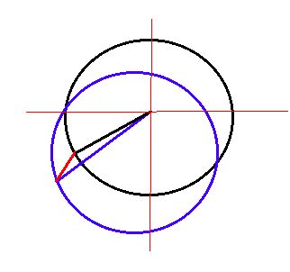
Hard Iron Error from Local Permanent Magnet
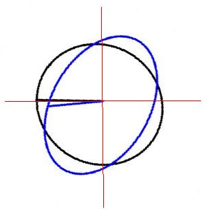
Soft Iron Error from Local Ferromagnetic Materials
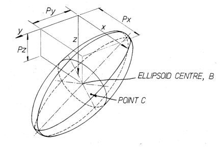
3D Ellipsoid from Marchent & Foster patent, 1985
3D Compass
I worked in analysis of torpedo sonar data at the Point Loma Naval Oceans Systems Center (1982-84). I also was part of a startup group at RD Instruments (1984-89) that developed the first doppler sonar ocean current measurement instruments (ADCP). There are generally more than three sonar beams in these systems and they definitely are not aligned with the instrument's xyz coordinates. In addition, the instrument body itself is not aligned with the earth's coordinates (shipboard systems and bouys). I developed a least squares method to project an arbitrary array of instrument sensors onto a given definition of x, y, and z.[8] So, when I encountered the 3D magnetic sensor array I immediately recognized that there was no theoretical constraint on the mounting of the sensors. A valid body-centered coordinate system could always be projected out from the sensor coordinates. In addition, once that coordinate system was defined it would be possible to project a north pointing vector onto a horizontal plane in that coordinate system.
Discontinuity
We get our direction by projecting the forward vector of our instrument onto the horizontal plane and measuring the angle between the projection and the north pointing vector. At high pitch angles the projection gets noisy; at 90 degrees it is undefined; at 91 degrees it flips sign. We handle these extreme cases by redefining what we consider forward. For example, patent 7103471 handles the case of a person-mounted compass when the user lies down on his stomach. In our person-mounted navigation systems we modeled the sensor as in the center of a cube with the sensor coordinate axes centered on the six faces. The user could specify any of six faces as the down direction. Of the four vertical faces, he could choose one for forward. Twenty four unique mounting orientations seemed to be enough for any user.
Temperature Compensation
Temperature affects sensors. It took a while to understand this. Our original compasses stored internal compensation tables that would correct the compass errors at a given azimuth. In between directions were interpolated. The problem was that by the time one got the table into memory, the self-heat from the device would corrupt the readings. Grrr!.
A simple way to test this is to heat the device with a hair dryer and then stick it in the freezer. Record sensor output as the temperature drops. Many sensors will have built-in temperature outputs, or one can use a dedicated sensor on the circuit board.
The plot below is from one such test. Notice how the sample points bunch at the lower end as the cooling rate decreases.
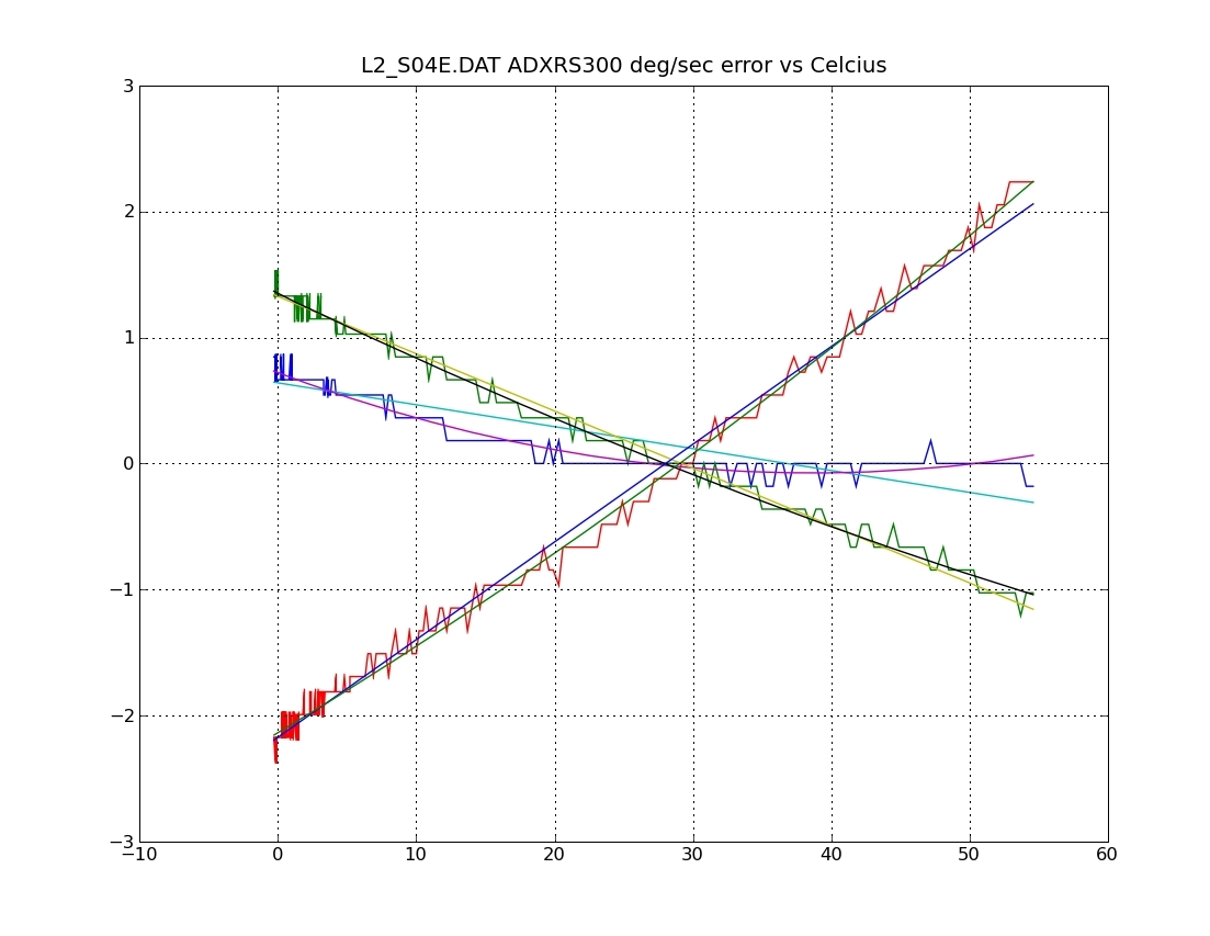
The above demonstrates temperature effects with the gyros. Remember the other sensors too: 3D accelerometers and magnatometers. Just collect the data from these sensors too as you are swinging the device through the temperature range.
Temperature response is usually NOT linear. There always seems to be some curve. One might then be suspicious of a temperature compensation algorithm that interpolated between just two data points. I have tried both two and three point routines. I did not find that the extra data point was worth the effort. Temperature calibrations dramatically increase manufacturing costs. So, reducing the length of time and the number of steps required to get the device calibrated is generally a good thing.
Iterative Solutions
I developed our iterative compass calibration algorithm from 1994-1998 at Point Research, Inc. I saw that a polynomial solution took a lot of work. I was interested in something that could be developed quickly and easily. I decided on an iterative process where the parameters are jiggled a little at each step. The best fit parameters are selected for the next round. The iterations are stopped with a convergence criterion that checks to see if there is any significant improvement.
But that is not all! I also dispensed completely with the polynomial and went directly to the offsets and transformation matrix. That is, the three offsets and nine elements of the 3x3 transformation matrix are the parameters I seek, not the ellipsoid polynomial coefficients. For the classical solutions, the matrix is symmetric, so there are only nine unique parameters. For high precision compass calibrations, we use all twelve parameters.
A side feature of this approach is that it circumvents the need to solve the eigenvalue/eigenvector problems. While this is a one-liner in MATLAB, it is not as easy in small embedded systems.
Precision Compass Calibration
Classic calibration of a magnetic compass can give you a compass with as low as a one degree error.
This is about as good as you can get when you use only the magnetic field samples.
Bob M., a co-worker at Point Research, applied additional
constraints using a calibration table. He was able to achieve better than one degree accuracy in the factory.
Gnepf and Weilenmann [7] showed how to include additional constraints from the accelerometers.
Their constraint is that the angle between the magnetic field and the gravitational field be constant.
I have tried a number of constraints that mix the accelerometer and magnetometer data:
- constant dot product
- constant magnitude of cross product
- constant magnitude of the determinant of the outer procuct
Shortcut Calibration
Tom's 3D Compass Calibration Shortcut
- Solve iteratively for the offsets and transformation matrix.
Below, a sample calculation on noisy, simulated data demonstrates the possibilities for precision iterative calibrations. Reproducible accuracy of better than a quarter degree sigma is possible.
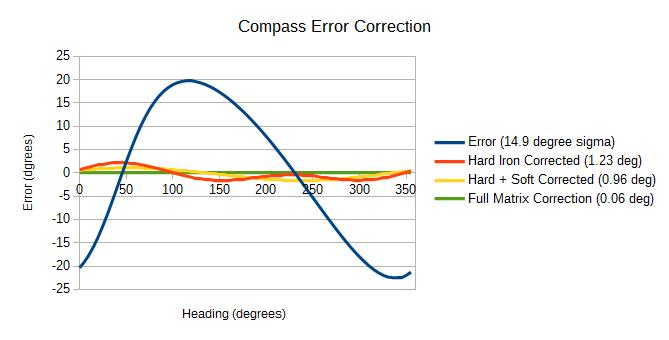
Iterative Calibration
Blue: Original Error
Orange: Hard Iron Error Corrected (3 parameters)
Yellow: Hard plus Soft Iron Error Corrected (9 parameters)
Green: Full Precision (12 parameters)
Iterative convergence is fairly slow, but quite acceptable for factory calibrations. I tried moving the calibration to the embedded system but it took minutes and minutes to converge. One final improvement by another co-worker, Eric E., sped up the calibration algorithm. He linearized the problem. Usable answers came with only a few iterations. I saw that we could now put the calibration in our compasses. The new calibrations took seconds to produce fractional degree results. Users could attain near-factory accuracy in the field [3].
References
- See US Patents 5583776, 7103471, 7890262, 8108171, 8423276, 8548766
- Judd, T., A Personal Dead Reckoning Module
- Judd, T., and Vu, T., Use of a New Pedometric Dead Reckoning Module in GPS Denied Environments
- Marchent and Foster, Compass, US Patent 4,539,760
- Fitzgibbon, Pilu, and Fisher, Direct Least Squares Fitting of Ellipses
- Halir and Flusser, Numerically Stable Direct Least Squares Fitting of Ellipses
- Gnepf and Weilenmann, Process for determining the direction of the earth's magnetic field, US Patent 6,009,629
- Judd, T, Outlines of Coordinate Transformations RD Instruments, 1989
- Kaiser,H.F., The JK method: a procedure for finding the eigenvectors and eigenvalues of a real symmetric matrix
©2022 Tom Judd
www.juddzone.com
Carlsbad, CA
USA