Magnetic Compass Calibration Sampling and Accuracy

Two Rules : Obtain accurate calibration with a simple guide for data collection
Background data collection : Calibrate a compass with data obtained while in use
Bunching/Excluding : Poor sampling can lead to bunching or unnecessary exclusion of data points
Quality Check : Validate with historical results during calibration to catch changes that impact accuracy.

Calibration Data Sampling

It is critical to follow these Two Rules when acquiring data samples for magnetic compass calibration:

Oversample the data. More than the minimum number of points is taken so that a few bad points do not bias the solution
Distribute the samples throughout the space of the problem. For example in a circle, collect samples more or less evenly around the circumference. Bunching samples on one side leaves the solution unconstrained on the other side. You then allow the solution to bulge or contract on the unconstrained side

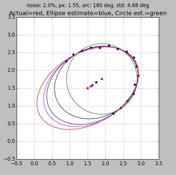
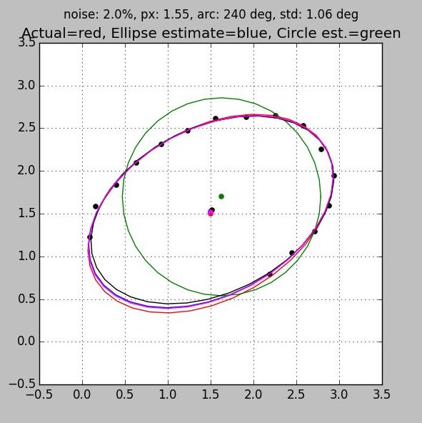
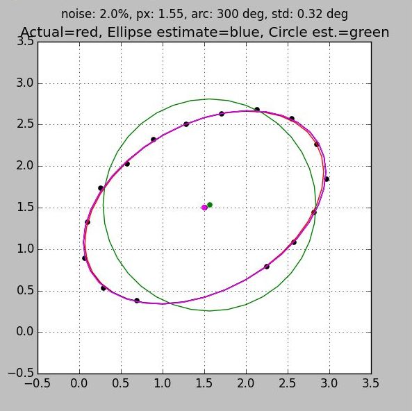
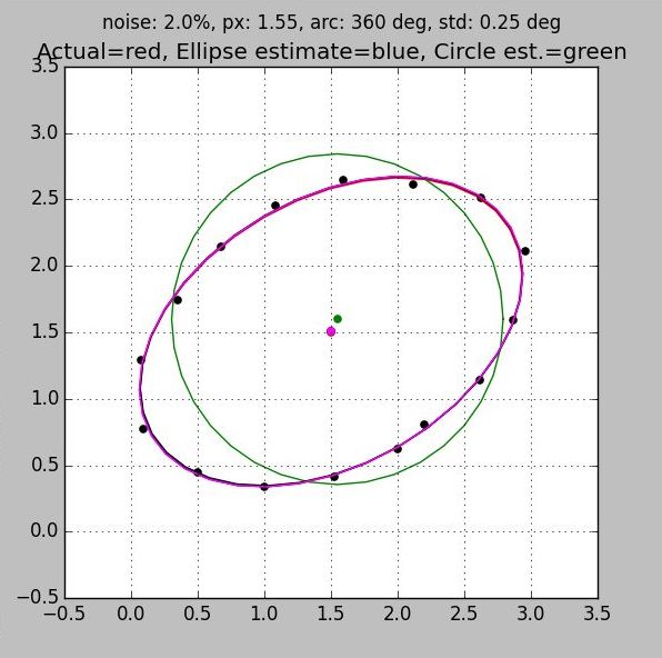
Both of these rules are demonstrated in the series of plots below which range from 50% coverage (Fig 1) to 100% coverage (Fig 4). Three separate ellipse algorithms are shown along with the best fit circle and the truth plot for reference:

Red: truth
Magenta: 2D iterative symmetric solution similar to the 3D Ellipsoid case.
Blue: Constrained Ellipse from Fitzgibbon (see references)
Black: Least Squares Ellipse ls_ellipse.py (see code)
Green: Least Squares Circle ls_circle.py (see code)

Features to notice are:

All plots have the same number of samples, but the first, which clumps the samples on one side of the ellipse, exhibits more than ten times the error than the last. This is due entirely to poor sample distribution
You can see the jitter in the sample points. But because all samples are used to arrive at an answer the solution benefits from averaging. Notice that with good sample distribution the error in the location of the center is much less than the individual sample error.
All algorithms converge to the same answer when the data is well distributed. They come so close that in the last two figures the ellipses are on top of each other giving the appearance of a single trace.
When a complete set of data is taken around the ellipse then the circle algorithm provides a very good estimate of the center.

This last point is important in iterative solutions. I have found that that the solution starts to diverge if the initial center is more than a third of the radius. The circle (or sphere in 3D) is just about the simplest algorithm presented here. The closed form solution does not require an eigenvector solution to find the center and radius. You get a good and easy estimate of the center from which to start the iterations. Also, since the circle (or sphere in 3D) algorithm is simple and robust, if it fails, then it is an indication that you probably need better data.

Calibration Accuracy

There are 360 degrees in a circle. If you want a precision compass that gives fractional degree accuracy, then you need at least one tenth of a degree accuracy. That is one part in 3600 accuracy. Twelve bits is 4096, just a bit over 3600. So it looks like you would need at least 12 bits of information. Convenience should allow for a sign, and the range should allow for strong external magnetic fields. So it looks like 14 bits is about the minimum you need for a precision compass. (M. Caruso in Magnetic Sensors in Low Cost Compass Systems.pdf came up with 12+ bits for 0.1 degree using an alternate analysis)

Quite early I decided that neither degrees nor radians were a satisfactory method of representing angles. I scaled the angle range 0..360 to 0..65536. Sixteen bit integers have features that make them suitable for expressing angles:

You can use the sign bit to indicate +/- 180
Like angles, the integer wraps at 360
Resolution is 0.006 degrees, twenty times better than we need for a precision compass

The units I called KANG for 64K ANGle. It has an advantage when using table lookup and extrapolation to calculate transcendental functions. For example, a cosine function with 64 entries can use the top six bits to get the closest table entry. We multiply the difference between that entry and the next with the remaining bits. The result is the cosine of an angle with only a single integer multiply. Everything else is shifts and adds.

I have used both integer and floating point solutions. Tests show that the integer truncation error is about 0.04 degree. The integer math is very fast. Table lookup and extrapolation for sine, cosine, arctangent, and square root contribute to the speed. All the compass calculations, filtering the three components of accelerometers, magnetometers, and gyros, coordinate system translation, temperature correction, and barometric altimeter calculations can be accomplished easily between samples (20msec @ 50Hz). We can be a bit lax here because we only need to maintain 14 bits of data. I made sure that all functions had 16 bits of accuracy.

When you have a compass with fractional degree accuracy you do not want the accuracy to be less after a calibration. We can adopt a 'sour grapes' calibration strategy. If the calibration crashes on bad data, then it surely would have decreased the accuracy even if it had succeeded. This gives us some leeway to take some shortcuts that would not be acceptable in the general sense. For example, our matrix inversion routine does not have to consider pivoting in order to maintain sixteen bit accuracy.

These algorithms have been around for some time. If you have difficulty with convergence, then most likely you have bad data

Background Sampling

Distributing samples for magnetic compass calibration is easy when done in the factory. The user can position the package in one of a set of predefined orientations, click the mouse OK, then proceed to the next point. In the field, the user may sometimes do the same, but without the benefit of a turntable. But when the challenge is to acquire samples in the background, while the device is in use, the problem may become unsolvable in some cases. For example, for devices fixed to a vehicle, most samples will lie in a horizontal plane. You cannot calibrate a 3D compass with samples that are confined to a single plane.

You actually need data from more than two independent planes in order to solve for a 3D ellipsoid. See the Degenerate Ellipsoid note for the reason why.

For a 2D solution we need at least 5 samples, sixteen would be oversampling by more than a factor of three. At a 50Hz sample rate, all our sample bucket would be filled in a fraction of a second. They would be clumped all together since there would be no time to significantly change the orientation of the magnetometers. There needs to be a means of spreading them out.

Time

The simplest strategy is to collect data over a period of time. This is useful during development when you have control over motion of the magnetometers: start, then turn the compass 360 degrees within the next 3 or 4 seconds. You usually get complete coverage if you are skilled. But it wastes memory with a lot of unneeded samples. You do not want to trust customers with this method.

Binning

A simple method that is customer friendly is to divide the circle up into bins. Just fill the bin with the sample when the calculated azimuth falls within the limits of the bin. If angles are expressed as KANG's then the upper n bits form an index into a 2ⁿ array of samples. Start the calibration computations when at least n/2 samples are taken and there is at most one empty bin between samples. You have to use an extra level of indirection to get this to work in 3D, otherwise your samples will bunch up at the poles. This method and the following Angle Separation method need a friendly environment in order to work because we are using the azimuth estimate in order to calibrate the azimuth.

Angle Separation

I had thought that a good set of 3D samples could be taken by simply making sure that the angle between it and all previous sample vectors was greater than some threshold. The dot product is an easy and obvious choice for calculating the angle. In 2007 I tested the scheme in MATLAB with excellent results. So, I moved it to our mobile platform. The C code comments simply describe the sampling strategy:

// index of vector with smallest dot on any previously picked vector
      . . .
// compare jtrial to all previously selected trials

It failed miserably in practice. The problem is that with strong hard iron effects, the offset can be larger than the radius. This puts the center from which angles are measured outside the circle of data. The plots show how Exclusion zones will then be created. Otherwise valid data points are rejected creating large undesirable gaps in the data. Even milder hard iron effects can lead to sample Bunching. This conflicts fundamentally with the goal of the sampling strategy which is to spread the samples evenly throughout the space of the problem.

I immediately went to Distance Separation below.

Degenerate* Ellipsoids

A spherical calibration takes magnetic field samples in 3D and finds the transformation that places all the points on a sphere:

X² + Y² + Z² = R² eq. 1

One scheme for sampling is to use two rotations about different axes. In the best orientation, the earth's field will sweep in a circle entirely within the plane perpendicular to the axis. For example, if we rotate about the X axis with that axis aligned east and west, then the X component of all the samples should be zero and all the samples should sweep out a circle in the YZ plane:

Y² + Z² = R² eq. 2

One can perform a similar rotation about the Y axis with it aligned east and west. This time the Y component is zero for all samples.

X² + Z² = R² eq. 3

This 3D data is insufficient for finding the solution to a 3D ellipsoid. To see this one only needs to consider a simple ellipsoid of the form

X² + Y² + Z² + K(XY) = R² eq. 4

When X is zero as it was in our first rotation, it reduces to equation 2; when Y is zero it becomes equation 3. The XY term drops out! The K coefficient of the XY term shows that there is a whole family of elliptical solids that can have circular intersections in two separate planes. Therefore, one cannot find a unique solution to a general ellipsoid from samples confined to these two planes.

*In quantum mechanics, an energy level is said to be degenerate if it corresponds to two or more different measurable states of a quantum system

A simple ellipsoid that demonstrates the problem is shown below. The ellipsoid that follows the equation X² + Y² + Z² + XZ = 1 cannot be distinguished from a unit sphere ( X² + Y² + Z² = 1) based on data confined to the two planes: XY (Z=0) and YZ(X=0).

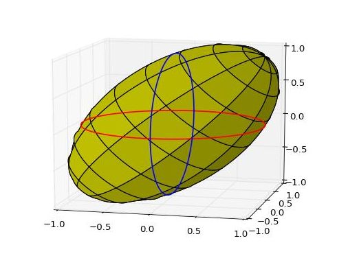
X² + Y² + Z² + XZ = 1 showing the circular intersection of the ellipsoid with the xy plane (red) and with the yz plane (blue)

Angle Separation Problem: Sample Bunching

Under mild conditions the technique is prone to bunching of samples. Below is a figure from Patent 8374816 which demonstrates how easily eight samples can be taken using Angle Spreading. These are highlighted by the eight green dots on the right of the figure. Overlooked in the patent is the fact that you do not know the character of the anomaly before you start taking samples. Instead of starting where sample 252-1 is shown, you could have just as easily started 180 degrees away on the other side of the circle. In fact, the lines for each of the samples could be extended in the opposite direction forming a complete alternate set of data. The result would be a clump of samples highlighted in red. We followed the algorithm, nothing changed except the starting point. But the result was just the opposite of what Angle Spreading is intended to do.

Excluded samples

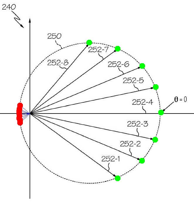
Sample selection by Angle Separation:Bunching problem. Figure adapted from Patent 8374816

Angle Separation Failure: Sample Exclusion

Using Angle Separation as a criterion, one rejects all the samples between the green arrows 1 and 2 in the figure because they are too close to sample 1. Sample 2 is accepted because it is over the minimum separation threshold from sample 1. However, on the near side, sample 3 would be excluded because the angle between it and either samples 1 or 2 is below the minimum separation. Selecting 1 and 2 on the far side creates an exclusion zone (in red) on the near side. As more samples are qualified along the far green arc, the corresponding exclusion region (in red) is is extended on the near side. This is a terrible and unnecessary sampling strategy.

Excluded samples

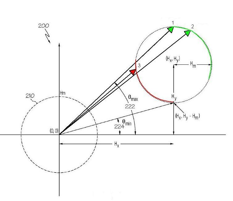
Sample selection by Angle Separation Fails; excludes half the ellipse (red zone). Figure adapted from Patent 8374816

Distance Separation

By far the most successful 2D and 3D background sampling scheme is to select points that are separated by a distance greater than some threshold. The technique is origin independent, so it works under mild or strong external fields. As soon as I observed the failure above with my Angle separation technique, I tried distance separation. It is actually easier to calculate: you do not have to normalize your vectors, and square roots seem more friendly than arc cosines. Although, it should be noted that the functions are monotonically increasing or decreasing in the region of interest. So, for example, a threshold based on the cosine of an angle will do as well as one based on the angle itself. Similarly, the square of a threshold value will work just as well when compared to the square of the distance (you don't have to use the square root).

The Distance Spacing Sample figure demonstrates the benefit of using a distance measure over an angle measure. We use the same diagram that depicted the bunching problem with an angle measurement algorithm. Starting from Sample 8, we continually search for sample vectors whose distance is greater than some threshold from all the previous samples. Sample 9 is selected because the distance between the tips of arrows 8 and 9 meets that criterion. We continue on around selecting samples 10, 11, and 12. Notice that the distance algorithm easily skips over the bunching region that plagued the angle separation algorithm.

Distance Spacing Sample

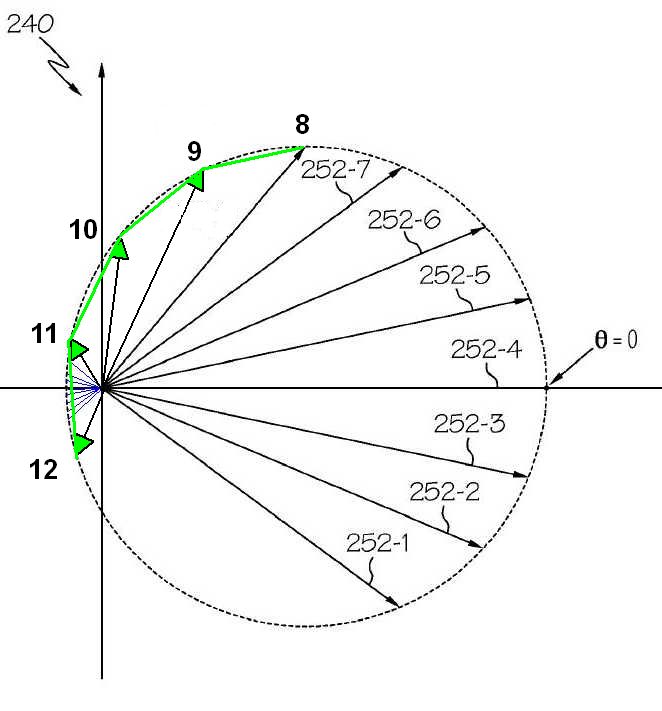
Sample selection by Distance Separation. Origin independent so segments are selected evenly where angle separation caused bunching.

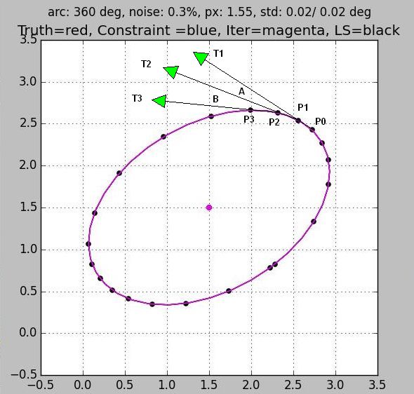
Curvature Separation

Selection of data samples by monitoring the curvature of the ellipse allows one to take a complete data set with a single spin of the compass. No a priori knowledge of the ellipse is needed.

The curvature of the ellipsoid can be detected by three points along the rim. Given that the first two points are chosen, the third has to be far enough away so that the vector between points 2 and 3 is at least a minimum angle from the vector between points 1 and 2. In the figure we show four successive points P0 through P3. They form three tangents, T1, T2, and T3. We space the point P2 such that the angle A between T1 and T2 is greater than some threshold angle. Once we have selected P2 we continue on to the next point. Point P3 should be chosen such that the angle B between T3 and T2 is also greater than some minimum. We continue in this manner until we have selected points all around the ellipse. The number of points is determined by the angle between the tangents. Picking 20 degree tangents will generate 360/20 or 18 sample points. Starting the whole process requires two points. This is easy. We just take the first sample and pick some conservative separation value for the second. In the figure you can see the first two points at the bottom right in the figure. They are close together because it is safer than accidentally leaving a large gap.

Our customers had been having trouble with our existing 2D field calibration procedure. Curiously, that procedure took TWO sets of data. The first was to determine the hard iron offsets. Once the offsets were determined the first data set was discarded! The user then turned the compass a second time, acquiring a whole new set of data points. The offsets obtained from the first set were subtracted from each data point in the second so binning or angle separation could be used to select the next set of points. All the data from the first set was thrown away. This is a terrible sampling method. It forces the developer to design two separate but tandem calibrations, and forces the user to do twice the work. No wonder they complained! It took me about ten minutes and the back of one envelope to come up with a single spin method that spaced samples predictably. The algorithm shown here is another improved single spin procedure.

If you are calibrating a 3D compass in 2D then the cross product can be used to measure the angle separation of the tangents, and provide a quality measure for the data. All vectors created by the cross product should be parallel if all the samples are in the same plane. Average all the cross product vectors, then use the deviation as the quality measure.

A drawback of this curvature technique is that it doesn't generalize to three dimensions easily.

Curvature Spacing Sample

Distance Separation

Sample selection by Curvature. Origin independent. Segments are most dense where the figure curves the most.

Quality Database

We started small. Then grew. As the volume of product increased it became clear that we had to change the access to our data. The data was there; but each device had its own data file in human readable form. So, it took a human to find and use the data. When a customer called with even the simplest of questions, it took a major effort just to find out the configuration of his system.

There was lots of data. Each compass had the obvious magnetic compass calibration coefficients. But in addition, each sensor for each axis had its own offset and gain that could be used to convert from the A/D counts to useful data values. Potentially, each component of each sensor had temperature coefficients and parameters for temperature calibration. Accelerometer, magnetometer, and gyro all had three axes. So, multiply by nine every parameter you can think of. We quickly blossomed to over a hundred calibration parameters. Add to that the test results (e.g. accuracy at level, accuracy at tilt, accuracy when rotated, etc.) and we could easily get to 200.

We did not want to rewrite all our code just so that we could generate a tractable data base. A clean way to handle this was to keep the existing code and data and write a script file that interfaced to the existing data files. We could then create a composite data file that had all the data from all the devices of a given type. So, that is what I did.

Each product had different parameters of interest. We eventually cloned the initial code to handle all our products.

Now I have a confession to make. I wrote it in Perl. Clearly, C is not a language that adapts itself easily to string manipulation. Better, I thought, to use a language that excelled in parsing text files. I had recently gone through Perl by Example and I thought this would be a good learn-by-doing opportunity.

It worked. But, I was not pleased with the experience. You who are familiar with Perl know all the pros and cons; so, I will leave it at that. Do-over would be in Python or C# both of which have good text manipulation features with fewer of the structural drawbacks.

Quality Check

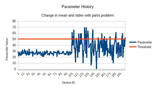
The Quality Database was wonderful. It could be read immediately into a spread sheet. Mean, standard deviation, and trend could be seen on all the parameters. We could now automate the quality checking that had been done manually, and we could do a more thorough job. Instead of just collecting 150 parameters, we could compare the parameters to historic values.

There had been a long standing need to check parameters as soon as they were generated. If there were an error, we would want to address it before anything else was done. More than once did errors happen and all subsequent work on the device was wasted. We therefore added files that defined the allowable limits for each parameter. As data was extracted and saved during calibration, it was also compared to historical values.

This was a very sensitive tool. Each parameter is linked in some way to the hardware. So, even small changes in hardware can result in detectable changes in the parameters. With acceptable hardware, there is a natural variation in the mean. And when the hardware changes, you will see a jump in the mean and/or standard deviation of the parameter. If the jump is outside the historical limits, then it calls for investigation. We have had expensive failures that would have been detected if the tool had been in use. So, even though I would have liked to have done a cleaner job writing the code, I was very pleased with the power it gave us in improving the overall quality of our products.

Parts History